Quantum Mechanics
Schrodinger equation
Quantum Mechanics
Propagators : Pg
Quantum Simple Harmonic
Oscillator QSHO
Quantum Mechanics
Simulation With GNU Octave
© The scientific sentence. 2010
|
|
Quantum Mechanics
Simple harmonic oscillator
Imaginary time
% ---------------------------------------------------
%personal
%addpath("C:/Octave/Octave-4.0.0/myfiles");
%qsho_code
% © TheScientificSentence.net
%-----------------------------------------------------
%Propagation in imaginary time of the simple harmonic
%oscillator calculation with non dimension parameters
%Gnu Octave or Matlab code .
%
% The related graphs shows the evolution of the wavefunction
%in imaginary time at different time steps. It converges from
%a wide gaussian initial arbitrary value to the gaussian ground
%state.
%----------------------------------------------------------------
% Clearing ------------------------------
clc
clf
clear all
%---------------------------------
kin = 0.067 ; %kinetic energy
% Space parametres -------------------
Lx=20; %length of x
Nx=10000; %number of x data points
dx=2*Lx/Nx;
x=(-Lx:dx:Lx-2*Lx/Nx);% x-coordinate
kx=pi*[0:Nx/2 -Nx/2+1:-1]/(Lx);% wave vector
k2xm=kx.^2; %wave vector squared
%Time -----------------------------
tf=0.1; %total time
dt=0.001; %time step
NL=tf/dt;% number of time loops
%Potential ---------------------
beta= 5; %beta^2 = mw^2/2
NumAtoms = 10^4;
V= beta^2 * x.^2;
% Other parametres ----------------------
alpha = 100; % mw/h_bar
u=(1/sqrt(pi*alpha))*exp((-.5/alpha)*(x.^2)) ;
u0 = u;
%initializing ---------------------------------
pot=0; E=0; Mu=0; Ur=0; T=0; m=1;
%split opperator method ----------------------
for n=0:NL-1
v=fft(u); % fourier transform
vna=exp(-0.25*kin*dt.*(k2xm)).*v;
una=ifft(vna);
pot=V ;
unb=exp(-1*dt*pot).*una;
vnb=fft(unb);
v=exp(-0.25*kin*dt.*(k2xm)).*vnb;
u=ifft(v);
% Renormalizing the function --------------
intv=sum(u(:).^2)*dx;
u=(u)./sqrt(intv);
if(mod(n-1,10)==0)
figure(1); clf;
h= plot(x,abs(u).^2);
set(h(1),'LineWidth',2);
xlim([-Lx Lx]) %axes
drawnow;
end
%energy --------------------------------------
dk=dx/(Nx);
Kn=sum( abs(k2xm.*fft(u).^2) )*kin*dk/2; %total kinetic energy
E1=V.*u.^2;
E2=sum(E1)*dx;
E(m)=real(Kn+E2);
E5(m,1)=m;
E5(m,2)=E(m);
end
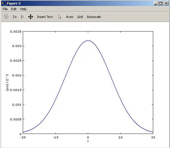
%Ploting of the probability density
figure(3);
plot(x, u0.^2) ;
xlabel('x','Interpreter', 'LaTex')
ylabel('|psi(x)|^2', 'Interpreter', 'LaTex')
% ----------------------------------
The output at a certain time :
|
|