1.Introduction

In the real microscopic world, it does not exist a particle alone inside any space. Dirac relativistic equation or Schrodinger's equation inform us about the single electron behavior in an atom. But when it come to try to do so with many electrons, the issue turns out to be very complicated. Kinetic theory of gases tells us that the internal energy of a gas is function of the temperature (more precisely U = (3/2) NkT, derived from the calculation of the mean square of the particle's speed) and involves only macroscopic terms. But what about the energy of each particle in the gas?. The only convenient way is to take the system as a whole, as an ensemble and studying in-depth this system statistically whereby to understand the structure of this matter by knowing how the energy is distributed among the particles. That is the purpose of the Statistical Mechanics

What do then "microscopic" and "macroscopic" stand for?
When one specify all the parameters of a particle of a system, we have a microstate for this system. Whereas, when a "global" situation of a system is considered, a kind of "snapshot" of the situation, we have a macrostate for this system.

2. Macrostates & Microstates


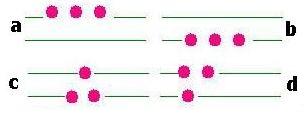
Let's consider the following example: We have 3 particles and 2 energy levels. If the particles are indistinguishable, we have then 4 configurations.

If the particles are distinguishable, we have 8 configurations.


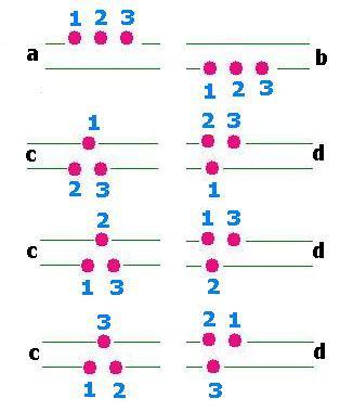
The number of macrostates is
4: Ω(a), Ω(b),Ω(c),Ω(d).
The number of microstates is
1 for Ω(a) and for Ω(b), and 3 for Ω(c) and Ω(d).

Remark

In the case of indistinguishable particles, every macrostate has no microstate. Forethermore:
Ω(a) = Ω(b) = Ω(c) = Ω(d) = 1. In other words, the macrostate is the microstate.

Now, let's fix the energy of this system with three particle to be E. Particles can occupy the two energy levels n_i (i = 1, 2).
If E_i (i = 1, 2) is the value of the energy associated to the level i, then:
E = Σ n_i [i = 1, 2].
As the total number of particles is already fixed to be N (here N = 3), if the number of levels is n; we have:

E = Σ n_iE_i    N = Σ n_i     [i: 1 → n]

Now, having n_i particles in each livel "i", that determines the macrostate for the system, how many microstates do we have for this macrostate?
If n₁ is the number of particles that lodge in the level "1", the number of ways to have this occupation is the number of combinations for n₁ particles among N particles; that is :
C₁ = C(n₁, N) = N!/n₁!(N - n₁)!
Once this case is set; it remains (N - n_i) particles to consider.
If n₂ is the number of particles that lodge in the level "2", the number of ways to have this occupation is the number of combinations for n₂ particles among (N - n₁) particles; that is:
C₂ = C(n₂, (N - n₁)) = (N - n₁)!/n₂!((N - n₁) - n₂!
...
Finaly, if the last level contains n_n particles = N - n₁ - n₂ - ... - n_{n - 1}, then the numbers of ways to distribute hem in within the last level "n" is C_n = C(n_n, n_n) = 1.
In total, the number of ways we have is the product of all the combinations. That is:
C₁ x C₂ x ... x C_n = ΠC_i [i: 1 → n]
= N!/n₁!(N - n₁)! x (N - n₁)!/n₂!((N - n₁) - n₂! x ... x 1. = N!/n₁ x n₂ x ... x 0!= N!/Πn_i [i: 1 → n]
The number of ways to distribute N particles over n levels containing each n_i particles is Ω = N!/Πn_i [i: 1 → n]]

In the case of a level "i" has a degeneracy g_i; that is the number g_i subshells, we can place n_i particles within by g_i^n_i ways; Thus:
The number of ways to distribute N particles over n levels containing each n_i particles; with a degeneracy g_i for the level "i" is Ω = N! Π(g_i^n_i/n_i) [i: 1 → n]]

The configuration (n₁, n₂, ..., n_i, ..., n_n) represents a macrostate wich has Ω = N! Π(g_i^n_i/n_i) microstates

3. Maxwell-Boltzmann distribution

Suppose that we toss up two dimes. The ways that we an have are:
(heads, heads); (tails, tails); (heads, tails) or (tails, heads) because we distinguish the pieces. The probability for each case is 1/4. If instead we have two balls, red and yellow, then indistinguishable, we will have the case: (red, red); (yellow, yellow); (red, yellow) = (yelolow, red). The probability for each case is 1/4, 1/4, 2/4. We say that the last case is most probable.
We are interested in the most probable case. To find the most probable case from the expression of Ω we derive it with respect to the number of particles n_i and zero if in order to find the extrema which give the most probable configuration.
From the expression of Ω itself, we can not go further. Taking the its Neperian logarithm "ln" will simplify graetly the issues.
Ω = N!Π (g_i^n_i)/n_i!, thus:
ln (Ω)= ln N! + Σ [n_iln g_i - ln n_i!]
Using the Stirling's approximation ln x! = x ln x - x , we have:
ln (Ω)= ln N - N + Σ [n_iln g_i - n_i ln n_i + n_i] = ln N + Σ [n_i][ln g_i - ln n_i] = ln N + Σ [n_i][ln (g_i/n_i)]
Thus: ln (Ω) = Σ [(dn_i)(ln(g_i/n_i)) - dn_i]

ln N! = Σ ln x [x: 1 → N] = ∫ ln x dx [x: 1 → N] = xln x - x [x: 1 → N] = Nln N - N + 1 . Neglecting 1, we can write: ln n! = nln N - N. Example: For N = 100, we have ln N! = 364 and Nln N - N = 360; an error ≈ 1% !

We have the following constraints:
N = Σ n_i
E = Σ n_iE_i
Or :
N - Σ n_i = 0
E - Σ n_iE_i = 0

If ∂ln(Ω)/∂n_i = 0, a linear combination with the constraints gives also zero (method using constants called Lagrange multipliers).
Let's define then a new function F as follows:
F(n_i) = ln(Ω) - λ(N - Σ n_i) + β(E - Σ n_iE_i) = NlnN - Σn_iln n_i - λ(N - Σ n_i) + β(E - Σ n_iE_i)
To find the extrema, Its derivative is :
∂F(n_i)/∂n_i = 0 That is: - 1 - ln n_i + λ - β E_i = 0
Let's set: λ - 1 = α; then: - ln n_i + α - β E_i = 0 . Thus: n_i = exp[ α - β E_i]; and
N = Σ n_i = Σ exp[ α - β E_i] = exp[ α] Σ exp[ - β E_i] exp[ α] = N/Σ exp[ - β E_i]
Let's set:
Z = Σ exp[- β E_i]
called the partition function.
It follows that: exp[ α] = N/Z. We find the
Maxwell-Boltzmann distribution:

n_i = Nexp(-βE_i)/Σexp(-βE_i) = Nexp(- βE_i)/Z