Calculus III
Contents
3 Dimensional space
Partial derivatives
Multiple integrals
Vector Functions
Line integrals
Surface integrals
Vector operators
Applications
© The scientific sentence. 2010
|
|
Calculus III:
Double Integrals
1. Double Integrals
1.1. The vector equation of the plane
We have seen the definition of a definite integral for functions of single variables,
by using the Riemann sum.
The definition of a definite integral of a function of single variable is :
| | b | | | | | | n | |
| ∫ | | f(x) dx | = | limit | | | Σ | f(a + k Δx) Δx |
| | a | | | Δx → 0 | | | k=1 | |
Δx = (b - a)/n , and
k = 1, 2, 3, ...
Now we want to integrate a function of two variables f(x,y) . With functions of one variable we integrated over a region of 1D space R .
With function of two variables we will integrate over a region of 2D space R2.
If we are integrate over the interval [a,b] for the variable x, and over the interval [c,d] for the variable y, then for
the function of two variables f(x,y)we integrate over
the rectangle R = [a, b] x [c, d]
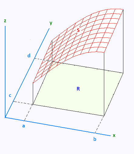
Let's consider the graph of the surface S given by graphing a function of two variables f(x,y) over the rectangle R.

The integrale of a function of one variable is the area under its curve. The integrale of a function of two variables is its volume under its curve.
The integrale of f(f,y) is the volume delimited by
the curve S and the rectangle R.
We divide up [a,b] into n subintervals and divide up [c,d] into m subintervals. This will divide up the rectangle R into a series of smaller rectangles and from each of these we will choose a point (a + iΔx, c + jΔy).
Over each of these smaller rectangles we will construct a box whose height is given by f(a + iΔx, c + jΔy).
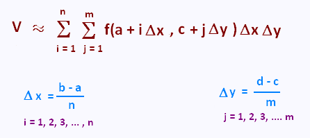
Each of the boxes has a base area of Δx Δy and a height of f(a + iΔx, c + jΔy). So the volume of each of these boxes is f(a + iΔx, c + jΔy) Δx Δy .
The volume under the surface S is then approximately

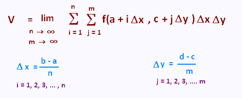
To get a better estimation of the volume we will take n and m larger and larger and to get the exact volume we will need to take the limit as both n and m go to infinity. That is

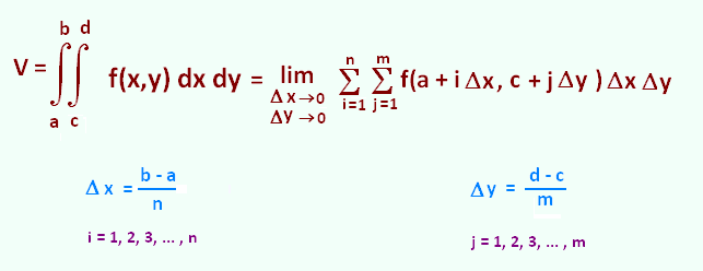
Finaly, all in one expression:

The double integral of f(x,y) over the rectangle R [a,b] x [c,d] is the volume under the function f(x,y) and above the xy-plane.
2. Computing Double Integrals : Iterated Integrals
Computing the integral, single integral or double integral Using the
definition with the Riemann sum, is often tedious. We need a technique to
actually compute double integrals.
We use, in practice, the method of iterated integrals. That is,
we integrate over a first variable, and then we repete for the second
variable.
Let's consider the function of two variables f(x,y) to integrate over the
rectangle R = [a, b] x [c, d].
We need to calculate
∫∫R f(x,y) dA
There are two ways, a similar process done with partial derivatives, to compute the integral:
• We think of all the x�s as constants and integrate with respect to y or
• we think of all y�s as constants and integrate with respect to x.
A first way is to integrate over the inner differential dx with its limits a and b, and then iterate for the outer differential dy with its limits c and d.

A second possibility is to integrate over the inner differential dy with its limits c and d, and then iterate for the differential dx with its limits a and b.

Fubini's theorem shows that the two ways leads to the same
results:

3. Examples
Example 1
∫∫R 2 x y dA, over the rectangle R = [2, 3] x [3, 8]
∫∫ R 2 x y dA =
∫23 ∫38 2 x y dx dy =
∫23 [∫38 2 x y dy] dx =
∫23 [∫38 2 x y dy] dx
We compute this by holding x constant and integrating with respect to y as if this were a single integral. This will give a function involving only x�s which we can in turn integrate:
∫38 2 x y dy = 2 x (y2/2)|38 =
2 x (1/2) ( 64 - 9) = 55 x
∫23 55 x dx = 55 (x2/2)|23 = 55 (1/2) (9 - 4) = 275/2.
∫23 ∫38 2 x y dx dy = 275/2
Example 2
∫∫R (x y2 + 1) dA, over the rectangle R = [0, 1] x [0, x]
∫∫ R (x y2 + 1) dA =
∫01 ∫0x (x y2 + 1) dx dy
To begin with, we integrate with respect to y:
∫01 [∫0x (x y2 + 1) dy] dx
[∫0x (x y2 + 1) dy] =
(xy3/3 + y)|0x =
x4/3 + x
Now over x:
∫01 [x4/3 + x] dx =
(x5/15 + x2/2)|01 =
1/15 + 1/2 = 17/30
∫01 ∫0x (x y2 + 1) dx dy = 17/30
Example 3
As the derivative by parts, we can do the integral in either direction. However, sometimes one direction of integration is significantly easier than the other.
Il is essential, before actually doing the integral, to make sure that the
taken way is the easier one .
∫∫R x exp{x y} dA, over the rectangle R = [0, 1] x [0, 1]
∫01∫01 x exp{x y} dx dy
To begin with, we integrate with respect to x:
∫01 [∫01 x exp{x y} dx] dy
∫01 x exp{x y} dx
The easier way is to do the following substitution:
u = x y , so du = y dx (y is taken constant)
∫ x exp{x y} dx =
∫ exp{u} du = exp{u} = exp {xy} . So
∫01 x exp{x y} dx = exp {xy}|01 = exp {y} - 1
Now over y:
∫01 (exp {y} - 1 ) dy =
(exp {y} - y)|01 = (e - 1) - (1)) = e - 2
Therefore:
∫01∫01 x exp{x y} dx dy = e - 2
4. Separable functions
A function of two independent variables is said to be separable if it can be expressed as a product of two functions, each of them depending on only one variable.
f(x,y) = g(x) . h(x)
So, if we can break up the function into a function only of x times a
function of y then we can do the two integrals individually and multiply them together. That is:

Example 4
∫∫R x ln(y) dA, over the rectangle R = [0, 1] x [1, 2]
∫01∫12 x ln(y) dx dy =
(∫01 x dx) (∫12 ln(y) dy)
=
((x2/2)|01) ((y ln(y) - y )|12 ) =
(1/2) (2ln(2) - 2 - (0 - 1)) =
(1/2) (2ln(2) - 2 - (0 - 1)) = ln(2)
Therefore:
∫01∫12 x ln(y) dx dy = ln(2)
|
|