Integral methods
1. Trapezoidal method
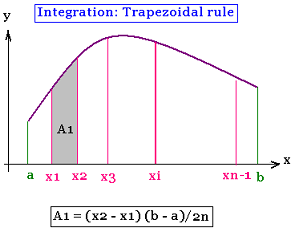
In this method, we divide the area under the curve
in trapezes.
A = Σ Ai
h = (b - a)/n
Ai = h [f(xi) + f(xi+1)]/2
I = A0 + A1 + A2 + ...
+ An-1
= h [f(a) + f(x1)]/2 + h [f(x1) + f(x2)]/2 +
h [f(x2) + f(x3)]/2 + ... + h [f(xn-1) + f(b)]/2
=
(h/2) [f(a) + f(x1) + f(x1) + f(x2) +
f(x2) + f(x3) + ... + f(xn) + f(b)]
=
(h/2) [f(a) + 2f(x1) + 2f(x2) + 2f(x3) + ... +
2f(xn-1) + f(b)]
=
h [(f(a) + f(b))/2 + f(x1) + f(x2) + f(x3) + ... + f(xn-1)]
=
h [(f(a) + f(b))/2 + Σf(xi) + ... + f(xn-1)]
i runs from 1 to n-1
A = h [(f(a) + f(b))/2 + Σ f(xi)]
i runs from 1 to n-1
xi = a + i h
x0 = a
xn = b
2. Rectangle method
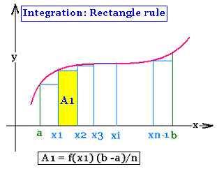
A = Σ Ai
h = (b - a)/n
Ai = h f(xi)
I = A0 + A1 + A2 + ...
+ An-1
= h f(x0) + h f(x1) + ... +
h f(xn-1)
= h Σ f(xi) i runs from 0 to n-1
A = h Σ f(xi)
i runs from 0 to n-1
xi = a + i h
x0 = a
xn = b
3. Midpoint method
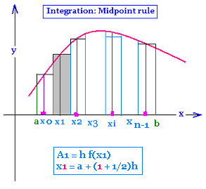
A = Σ Ai
h = (b - a)/n
Ai = h f(xi)
I = A0 + A1 + A2 + ...
+ An
= h Σ f(xi)
i runs from 0 to n
xi = a + (i + 1/2) x h
A = = h{[f(a) + f(b)]/2 + Σ f(xi)}
i runs from 0 to n-1
xi = a + (i + 1/2) h
x0 = a + h/2
xn-1 + (n - 1/2) h
x0 - h/2 = a
xn-1 + h/2 = b
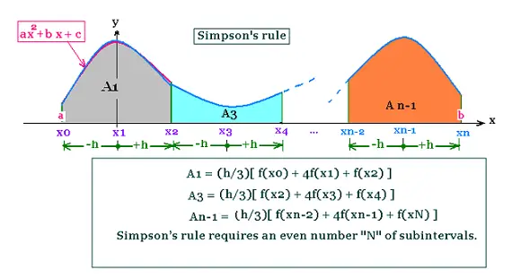
4. Simpson method
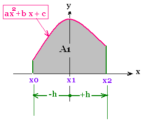
The area under the curve on the interval
[x0, x2] is approximated by a parabola y = ax2 + bx + c.
The total integral will be equal to the sum of all the area
under the set of parabolic arches.
A1 = ∫ (ax2 + bx + c)dx
from - h to + h
= (a/3)[+ h3 + h3 ] +
(a/2)[h2 - h2] + c[h + h]
=
(2a/3)h3 + 0 + 2ch =
(2a/3)h3 + 2ch
A1 = (h/3)[2ah2 + 6c ]
(1)
We have also:
f(x0) = f(-h) = ah2 - bh + c
f(x1) = f(0) = c
f(x2) = f(+h) = ah2 + bh + c
Then:
A1 = (h/3)[2ah2 + 6c ] =
(h/3)[ f(x0) + f(x2) - 2c + 6f(x1)] =
(h/3)[ f(x0) + f(x2) - 2f(x1) + 6f(x1)] =
(h/3)[ f(x0) + 4f(x1) + f(x2) ] =
A1 = (h/3)[ f(x0) + 4f(x1) + f(x2) ]
(2)
A = Σ Ai =
A1 + A3 + ... +
An-1
=
(h/3)[ f(x0) + 4f(x1) + f(x2) ] +
(h/3)[ f(x2) + 4f(x3) + f(x4) ] +
(h/3)[ f(x4) + 4f(x5) + f(x6) ] +
... +
(h/3)[ f(xn-2) + 4f(xn-1) + f(xN) ]
Simpson�s rule requires an even number "N" of subintervals.
A =
(h/3)[ f(x0) + 4f(x1) + 2f(x2) +
+ 4f(x3) + 2f(x4) +
+ 4f(x5) + f(x6) +
... +
2f(xn-2) + 4f(xn-1) + f(xN)]
Ai = (h/3)[ f(xi-1) + 4f(xi) + f(xi+1) ]
(3)
Therefore:
A = Σ Ai = (h/3)Σ[ f(xi-1) + 4f(xi) + f(xi+1) ]
i runs from: 1 to n
5.Gauss Quadrature rule
In this method, we equate the function to integrate f(x) to a
polynomial and integrate this polynomial that will be equal to
a linear combination of other simple functions.
Thar is:
∫f(x) dx (from a to b) = ∫ Σ aixi) dx
= Σ cif(xi)
i runs from 0 to n
∫ f(x) dx from a to b = Σ ci f(xi) i from 0 to n
xi is called weight, and xi: argument.
f(x) = a0 + a1 x1 + a2 x2 + a3 x3 +
... + an xn
= Σ ai xi i from 0 to n
Σ ci f(xi) i from 0 to n =
Σ ai xi i from 0 to n
c0 f(x0) = a0 x0
c1 f(x1) = a1 x1
c2 f(x2) = a2 x2
...
cn f(xn) = an xn
∫ f(x) dx from a to b = Σ ci f(xi)
= ∫ [Σ ai xi] dx
= a0(b - a) + (a1/2)(b2 - a2) +
(a2/3)(b3 - a3) + ... +
(an/(n+1))(bn+1 - an+1)
Then:
a0(b - a) = c0 f(x0)
(a1/2)(b2 - a2) = c1 f(x1)
...
(an/(n+1))(bn+1 - an+1) = cn f(xn)
Example:
I = ∫ (2 + 3 x2) dx from -1 to +1
f(x) = 2 + 3 x2
. Litterally, we have:
∫ f(x) dx = 2 [1 + 1] + 0 + 3 (1/3)[13 - (-1)3]
= 4 + 0 + 2 = 6
1. One point quadrature rule:
∫ f(x) dx = c1f(x1)
f(x) = a0x0 + a1x1
∫ f(x) dx from -1 to + 1 = a0 x 2 + a1 (1/2) [(1)2 - (-1)2]
= 2a0 + 0 a1 = 2a0
c1f(x1) =
c1a0x0 + c1a1x1
= 2a0
c1a0x0 = 2 a0
c1a1x1 = 0
c1x0 = 2
c1x1 = 0
c1 = 2
x1 = 0
For our example:
∫ f(x) dx = 2 f(0) = 2 x 2 = 4
The order one is not sufficient ...
2. Two points quadrature rule :
∫ f(x) dx = c1f(x1) + c2f(x2)
f(x) = a0x0 + a1x1 +
a2x2 + a3x3
∫ f(x) dx from a to b =
a0 (b - a) + (a1/2) [b2 - a2]
+ (a2/3) [b3 - a3] +
+ (a3/4) [b4 - a4]
c1f(x1) + c2f(x2) =
c1 [a0 + a1x1+
a2x12 + a3x13] +
c2[a0 + a1x2 +
a2x22 + a3x23]
(c1 + c2)a0 +
(c1x1 + c2 x2)a1 +
(c1x12 + c2x22)a2 +
(c1x13+ c2x23)a3
(c1 + c2)a0 +
(c1x1 + c2 x2)a1 +
(c1x12 + c2x22)a2 +
(c1x13+ c2x23)a3
a0 (b - a) + (a1/2) (a2 - b2)
+ (a2/3) (a3 - b3) +
+ (a3/4) (a4 - b4)
Therefore:
c1 + c2 = (b - a)
c1x1 + c2 x2 = (1/2) (b2 - a2)
c1x12 + c2x22 =
(1/3) (b3 - a3)
c1x13+ c2x23
(1/4) (b4 - a4)
Example:
a = -1 and b = +1, then:
c1 + c2 = 2 (1)
c1x1 + c2 x2 = 0 (2)
c1x12 + c2x22 = 2/3 (3)
c1x13+ c2x23 = 0 (4)
c1x1 = - c2 x2 (2)
c1x13 = - c2x23 (4)
Dividing (4)by (2) yields:
x12 = x22
Then:
x1 = +/- x2
If x1 = x2 then c1 - c2 = 0 No according to (2)
and we want these two arguments not null. Therefore:
x1 = - x2 and c1 = c2 = 1
Using (3)
c1x12 + c2x12 = 2/3 (3)
[c1 + c2]x12 = 2/3
Using (1)
x12 = 1/3 and x1= 1/31/2
Then:
c1 = c2 = 1
x1 = - x2 = 1/31/2
For our example:
f(x) = 2 + 3 x2
∫ f(x) dx = c1f(x1) + c2f(x2)
= f(1/31/2) + f( - 1/31/2)
= 2 + 1 + 2 + 1 = 6
That is the exact result.
First order : 4
second order: 6
3. General case:
∫ f(x) dx = Σ cif(xi) i from 1 to n
f(x) = Σ aixixi i from 1 to n
Then:
Σ ci = (b - a)
Σ cixi = (1/2) (b2 - a2)
Σ cixi2 = (1/3) (b3 - a3)
Σ cixi3 = (1/4) (b4 - a4)
....
Σ cixik = (1/(k+1)) (bk+1 - ak)
ΣΣ cixik = (1/(k+1)) (bk+1 - ak)
i from: 1 to n and k from: 0 to n+1
4. General case for integrations limits:
∫ f(x) dx from a to b, can be written as:
∫ f(x) dx from -1 to +1 by changing the variable x to X
x = (b - a)X/2 + (a + b)/2
Then:
dx = (b - a)dX/2, then:
∫ f(x) dx from a to b = [(b - a)/2]∫ f((b - a)X/2 + (a + b)/2) dX from -1 to +1
The Gauss n quardature rule is:
ΣΣ cixik = (1/(k+1)) (bk+1 - ak)
i from: 1 to n and k from: 0 to n+1
=
∫ f(x) dx from a to b = [(b - a)/2]∫ f((b - a)X/2 + (a + b)/2) dX from -1 to +1
With x = (b - a)X/2 + (a + b)/2
∫ f(x) dx from a to b = [(b - a)/2]∫ f((b - a)x/2 + (a + b)/2)dx
x runs from -1 to +1
= [(b - a)/2] Σ cixi
Where ci and xi are solved with a = -1 and b = +1 in the
equation:
ΣΣ cixik = (1/(k+1)) (bk+1 - ak)
i runs from 1 to n and k from: 0 to n+1
Example
I = ∫ (2 + 3 x2) , dx from -2 to +5
= [(5 + 2)/2]∫ f((5 + 2)X/2 + (5 - 2)/2), dX from -1 to +1
= (7/2)∫ f(7X/2 + (3/2)) dX from -1 to +1
= (7/2)∫ (2 + 3 [7X/2 + (3/2)2]) dX from -1 to +1 =
(7/2)∫ (2 + 3 [(49/4)x2 + (21/2)X +(9/4)]) dX from -1 to +1 =
(7/2)∫ (2 + (147/4)x2 + (63/2)X +(27/4)) dX from -1 to +1 =
(7/2)∫ ((147/4)x2 + (63/2)X +(35/4)) dX from -1 to +1 =
(7/2)((147/12)x3 + (63/4)X2 +(35/4)X) =
(7/2)((147/12)[1 + 1] + (63/4)[1 - 1] +(35/4)[1 +1]) =
(7/2)(252/6) = (7/2)(42) = 147
Litterally,
I = ∫ (2 + 3 x2) dx from -2 to +5 =
2[7] + (3/3)[53 - (-2)x3] =
14 + [125 + 8] = 147
We obtain the same result.
Now we will integrate by using Gauss' two quadrature order method:
I = ∫ (2 + 3 x2) , dx from -2 to +5
= (7/2)∫ (2 + 3X2), dX from -1 to +1
with X = (5 + 2)/2 x + (-2 + 5)/2 = 3.5 x + 1.5
Then:
c1 = c2 = 1
X1 = - X2 = 1/31/2
∫ f(x) dx = c1f(x1) + c2f(x2)
= (7/2) [f(3.5/31/2 + 1.5 ) + f( - 3.5/31/2 + 1.5)]
= (7/2) [2 + 3 (3.5/31/2 + 1.5)2 + 2 + 3(- 3.5/31/2 + 1.5)2]
= (7/2) [4 + 2 (3.52 + 6 (1.5)2]
= (7/2) [4 + 24.50 + 13.50>] = 147
We obtain the same result.
|