Probability

1. Poisson distribution

If the probability of one success is p; the probabily to get exactly 
n success among N trials is: 

P(n/N) = C(n,N)pnqN-n = [N!/n!(N-n)!] pnqN-n	(1)

N!/(N-n)! = N x (N-1) x (N-2) x ... x (N- n+2) x (N - n+1)	(2)

We define the parent parameter λ as:
λ = N x p
Where N is the number of trials, and p is the parent probability 
to get success.

The expression (1) becomes:
P(n/N) = [N x (N-1) x (N-2) x ... x (N-n+2) x (N-n+1)/n!] (λ/N)n(1 - λ/N)N-n	
= [N x (N-1) x (N-2) x ... x (N-n+2) x (N-n+1)/Nn] x 
[λn/n!] x (1 - λ/N)N x (1 - λ/N)-n	(3)

Now if N is large, the probability P(n/N) becomes:
pλ(n) = lim p(n/N) when n → ∞

pλ(n) = 1 x [λn/n!] x (1 - λ/N)N x 1 	(4)

Using Taylor Series:
ex = 1 + x + x2/2! + x3/3! +... (T1)
(1 + x)n = 1 + nx + n(n - 1)/2! x2 + ... 	(T2)
we have respectively:
e- λ = 1  - λ + λ2/2!  + ... 	(T11)
(1 - λ/N)N = 1 - λ + N(N - 1)/2!N2 λ2 + ...	(T22)

When N → ∞ N(N - 1)/N2 → 1 ; the relationship (T22) becomes:
(1 - λ/N)N = 1 - λ + λ2/2! + ...	
That is the relationship (T11)

Thus,
(1 - λ/N)N → e- λ

Finally, the relationship (4) becomes:
pλ(n) = [λn/n!] x e- λ


pλ(n) = λn e- λ/n!



More generally,

If we define the parent parameter λ as:
λ = N x p; where N is a large number of trials, 
and p is the parent probability to get one success 
(one event E); the probability of observing X = x; 
where X is the random variable, a disctete value 
that describes the number of times a given outcome 
occurs is:
p(X = x) = λx e- λ/x!



The Poisson distribution is a discrete distribution that characterizes 
the occurence of rare events. It is associated with counting experiments; 
such as radioactive decay.

The parent probability p is associated with one (success) 
outcome E, we can then write p = E(X)/N, where E(X) is the 
expected value for the random variable X related to the 
event E. The relationship λ = N x p becomes: 
λ = E(X)



Using again the Taylor seriess:
ex = 1 + x + x2/2! + x3/3! +... = ∑ xn/n!	(T1)
we sum the formula pλ(n) = λn e- λ/n! 
to obtain:
∑pλ(n) = ∑λn e- λ/n! 
= e- λ ∑λn/n! = e- λ eλ = 1

2. Poisson distribution Expectation value and variance

2.1. Expectation value

The expaectation value or mean for the Poisson distribution is:
E(x) = μ = ∑ x Po(x) [x: 0 → +∞]
= ∑ x μxe- μ/x! 	[x: 0 → +& infin;] 
= e- μ ∑ μx/(x - 1)! 	[x: 1 →+ ∞]
= e- μ ∑ μx+1/x! 	[x: 0 → + ∞]
= e- μ μ ∑ μx/x! 	[x: 0 → + ∞]

According to the expansion: 
eζ = ∑ ζx/x! 	[x: 0 → + ∞]
It follows:

E(x) = e- μ μ eμ = μ 

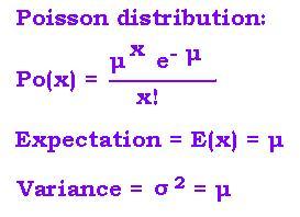
Poisson distribution: Po(x) = μxe- μ/x! 
Expectation = E(x) = μ

2.2. Variance

The variance of the Poisson distribution is:

σ2 = ∑ (x - μ)2 Po(x) [x: - ∞ → + ∞]
or 
σ2 = ∑ (x - μ)2 Po(x) [x: 0 → + n] 
for a large number n of measurements of x.
We have:
σ2 = ∑ x2 Po(x) - 2 μ ∑ x Po(x) +  ∑ x2 Po(x)
= ∑ x2 Po(x) - 2 μ2 + ∑2 
= ∑ x2 Po(x) -  μ2 
with x2 = x(x - 1) + x,
σ2  =  ∑ (x(x - 1) + x) Po(x) -  μ2 
=  ∑ (x(x - 1)) Po(x) + μ -  μ2 
=  ∑  μxe- μ/(x - 2)!) + μ -  μ2 
=  μ2 ∑  μx - 2e- μ/(x - 2)!) + μ -  μ2
=  μ2 ∑  μx - 2e- μ/(x - 2)!) + μ -  μ2 [x: 2 → + n] 

According to the expansion: 
eζ = ∑ ζx/x! 	[x: 0 → + ∞]
It follows:
∑  μx - 2/(x - 2)!) [x: 2 → + n]  
= ∑ μx /x! = 	eμ	[x: 0 → + ∞]

Then:
σ2 = μ2 e+μ e-μ + μ -  μ2 = μ

Poisson distribution: Po(x) = μxe- μ/x! 
Variance = σ2  = μ